PLUMED Masterclass 21.6: Dimensionality reduction
Aims
The primary aim of this Masterclass is to show you how you might use PLUMED in your work. We will see how to call PLUMED from a python notebook and discuss some strategies for selecting collective variables.
Objectives
Once this series of exercises is completed, users will be able to:
- Run dimensionality reduction algorithms with PLUMED
Resources
The data needed to complete this Masterclass can be found on GitHub. You can clone this repository locally on your machine using the following command:
git clone https://github.com/plumed/masterclass-21-6.git
I recommend that you run each exercise in a separate sub-directory (i.e. Exercise-1, Exercise-2, …), which you can create inside the root directory masterclass-21-6. Organizing your data this way will help you to keep things clean.
All the exercises have been tested with PLUMED version 2.7.0.
Acknowledgements
Throughout this exercise, we use the atomistic simulation environment and chemiscope. Please look at the information at the links I have provided here for more information about these codes.
Exercises
Chemiscope comes into its own when you are working with a machine learning algorithm. These algorithms can (in theory) learn the collective variables you need to use from the trajectory data. To make sense of the coordinates that have been learned, you have to carefully visualize where structures are projected in the low dimensional space. You can use chemiscope to complete this process of visualizing the representation the computer has found for you. In this next set of exercises, we will apply various dimensionality reduction algorithms to the data contained in the file traj.pdb. If you visualize the contents of that file using VMD, you will see that this file contains a short protein trajectory. You are perhaps unsure what CV to analyze this data and thus want to see if you can shed any light on the contents of the trajectory by using machine learning.
Typically, PLUMED analyses one set of atomic coordinates at a time. To run a machine learning algorithm, however, you need to gather information on multiple configurations. Therefore, the first thing you need to learn to use these algorithms is how to store configurations for later analysis with a machine learning algorithm. The following input illustrates how to complete this task using PLUMED.
# This reads in the template pdb file and thus allows us to use the @nonhydrogens # special group later in the inputMOLINFOThis command is used to provide information on the molecules that are present in your system. More detailsSTRUCTURE=__FILL__a file in pdb format containing a reference structureMOLTYPE=proteinwhat kind of molecule is contained in the pdb file - usually not needed since protein/RNA/DNA are compatible
# This stores the positions of all the nonhydrogen atoms for later analysis cc:COLLECT_FRAMES__FILL__=This allows you to convert a trajectory and a dissimilarity matrix into a dissimilarity object More details@nonhydrogensall non hydrogen atoms. Click here for more information.
# This should output the atomic positions for the frames that were collected to a pdb file called traj.pdbDUMPPDBOutput PDB file. More detailsATOMS=cc_datavalue containing positions of atoms that should be outputATOM_INDICES=the indices of the atoms in your PDB output@nonhydrogensall non hydrogen atoms. Click here for more information.FILE=traj.pdbthe name of the file on which to output these quantities
Copy the input above into a plumed file and fill in the blanks. You should then be able to run the command using:
Then, once all the blanks are filled in, run the command using:
plumed driver --mf_pdb traj.pdb
You can also store the values of collective variables for later analysis with these algorithms. Modify the input above so that all Thirty backbone dihedral angles in the protein are stored, and output using OUTPUT_ANALYSIS_DATA_TO_COLVAR and rerun the calculation.
You can find more information on the dimensionality reduction algorithms that we are using in this section in this paper.
PCA
Having learned how to store data for later analysis with a dimensionality reduction algorithm, lets now apply principal component analysis (PCA) upon our stored data. In principle component analysis, low dimensional projections for our trajectory are constructed by:
- Computing a covariance matrix from the trajectory data
- Diagonalizing the covariance matrix.
- Calculating the projection of each trajectory frame on a subset of the eigenvectors of the covariance matrix.
To perform PCA using PLUMED, we are going to use the following input with the blanks filled in:
# This reads in the template pdb file and thus allows us to use the @nonhydrogens # special group later in the inputMOLINFOThis command is used to provide information on the molecules that are present in your system. More detailsSTRUCTURE=__FILL__a file in pdb format containing a reference structureMOLTYPE=proteinwhat kind of molecule is contained in the pdb file - usually not needed since protein/RNA/DNA are compatible
# This stores the positions of all the nonhydrogen atoms for later analysis cc:COLLECT_FRAMES__FILL__=This allows you to convert a trajectory and a dissimilarity matrix into a dissimilarity object More details@nonhydrogens# This computes and diagonalizes the covariance matrix and projects each of the input coordinates into the low dimensional space # The output file here contains details of the eigenvectors that were obtained pca:all non hydrogen atoms. Click here for more information.PCAPerform principal component analysis (PCA) using either the positions of the atoms a large number of collective variables as input. More detailsARG=__FILL__the arguments that you would like to make the histogram forNLOW_DIM=2number of low-dimensional coordinates requiredFILE=pca_proj.pdb # This will output the PCA projections of all the coordinatesthe file on which to output the low dimensional coordinatesDUMPVECTORPrint a vector to a file More detailsARG=__FILL__the input for this action is the scalar output from one or more other actionsFILE=pca_datathe file on which to write the vetors
# These next three commands calculate the secondary structure variables. These # variables measure how much of the structure resembles an alpha helix, an antiparallel beta-sheet # and a parallel beta-sheet. Configurations that have different secondary structures should be projected # in different parts of the low dimensional space. alpha:ALPHARMSDProbe the alpha helical content of a protein structure. More detailsRESIDUES=all abeta:this command is used to specify the set of residues that could conceivably form part of the secondary structureANTIBETARMSDProbe the antiparallel beta sheet content of your protein structure. More detailsRESIDUES=allthis command is used to specify the set of residues that could conceivably form part of the secondary structureSTRANDS_CUTOFF=1.0 pbeta:If in a segment of protein the two strands are further apart then the calculation of the actual RMSD is skipped as the structure is very far from being beta-sheet likePARABETARMSDProbe the parallel beta sheet content of your protein structure. More detailsRESIDUES=allthis command is used to specify the set of residues that could conceivably form part of the secondary structureSTRANDS_CUTOFF=1.0If in a segment of protein the two strands are further apart then the calculation of the actual RMSD is skipped as the structure is very far from being beta-sheet like
# These commands collect and output the secondary structure variables so that we can use this information to # determine how good our projection of the trajectory data is. cc2:COLLECT_FRAMESThis allows you to convert a trajectory and a dissimilarity matrix into a dissimilarity object More detailsARG=alpha,abeta,pbetathe arguments you would like to collectDUMPVECTORPrint a vector to a file More detailsARG=cc2_datathe input for this action is the scalar output from one or more other actionsFILE=secondary_structure_datathe file on which to write the vetors
To generate the projection, you run the command:
plumed driver --mf_pdb traj.pdb
You can generate a projection of the data above using chemiscope by using the following script:
# This ase command should read in the traj.pdb file that was analyzed.  Notice that the analysis
# actions below ignore the first frame in this trajectory, so we need to take that into account
# when we generated the chemiscope
traj = ase.io.read('../data/traj.pdb',':')
# This reads in the PCA projection that are output by by the OUTPUT_ANALYSIS_DATA_TO_COLVAR command
# above
projection = np.loadtxt("pca_data")
# We also read in the secondary structure data by colouring points following the secondary
# structure. We can get a sense of how good our projection is.
structure = np.loadtxt("secondary_structure_data")

# This ensures that the atomic masses are used in place of the symbols
# when constructing the atomic configurations' chemiscope representations.
# Using the symbols will not work because ase is written by chemists and not
# biologists.  For a chemist, HG1 is mercury as opposed to the first hydrogen
# on a guanine residue.
for frame in traj:
    frame.numbers = np.array(
        [
            np.argmin(np.subtract(atomic_masses, float(am)) ** 2)
            for am in frame.arrays["occupancy"]
        ]
    )

# This constructs the dictionary of properties for chemiscope
properties = {
    "pca1": {
        "target": "structure",
        "values": projection[:,0],
        "description": "First principle component",
    },
    "pca2": {
        "target": "structure",
        "values": projection[:,1],
        "description": "Second principle component",
    },
    "alpha": {
        "target": "structure",
        "values": structure[:,0],
        "description": "Alpha helical content",
    },
    "antibeta": {
        "target": "structure",
        "values": structure[:,1],
        "description": "Anti parallel beta sheet content",
    },
    "parabeta": {
        "target": "structure",
        "values": structure[:,2],
        "description": "Parallel beta sheet content",
    },
}

# This generates our chemiscope output
write_input("pca_chemiscope.json.gz", frames=traj[1:], properties=properties )
When the output from this set of commands is loaded into chemiscope, we can construct figures like the one shown below. On the axes here, we have plotted the PCA coordinates. The points are then coloured according to the alpha-helical content.
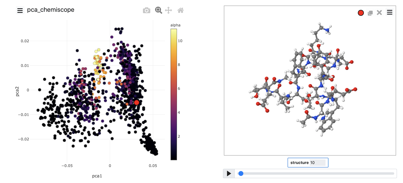
See if you can use PLUMED and chemiscope to generate a figure similar to the one above. Try to experiment with the way the points are coloured. Look at the beta-sheet content as well.
MDS
In the previous section, we performed PCA on the atomic positions directly. In the section before last, however, we also saw how we could store high-dimensional vectors of collective variables and then use them as input to a dimensionality reduction algorithm. Therefore, we might legitimately ask if we can do PCA using these high-dimensional vectors as input rather than atomic positions. The answer to this question is yes as long as the CV is not periodic. If any of our CVs are not periodic, we cannot analyze them using the PCA action. We can, however, formulate the PCA algorithm differently. In this alternative formulation, which is known as classical multidimensional scaling (MDS), we do the following:
- We calculate the matrix of distances between configurations
- We perform an operation known as centring the matrix.
- We diagonalize the centred matrix The eigenvectors multiplied by the corresponding eigenvalue’s square root can then be used as a set of projections for our input points.
This method is used less often than PCA as the matrix that we have to diagonalize here in the third step can be considerably larger than the matrix that we have to diagonalize when we perform PCA.
To avoid this expensive diagonalization step, we often select a subset of so-called landmark points on which to run the algorithm directly. Projections for the remaining points are then found
by using a so-called out-of-sample procedure. This is what has been done in the following input:
# This command reads in the template pdb file and thus allows us to use the @nonhydrogens # group later in the inputMOLINFOThis command is used to provide information on the molecules that are present in your system. More detailsSTRUCTURE=__FILL__a file in pdb format containing a reference structureMOLTYPE=proteinwhat kind of molecule is contained in the pdb file - usually not needed since protein/RNA/DNA are compatible
# This stores the positions of all the nonhydrogen atoms for later analysis cc:COLLECT_FRAMESThis allows you to convert a trajectory and a dissimilarity matrix into a dissimilarity object More detailsATOMS=list of atomic positions that you would like to collect and store for later analysis@nonhydrogensall non hydrogen atoms. Click here for more information.
# The following commands compute all the Ramachandran angles of the protein for you r2-phi:TORSIONCalculate a torsional angle. More detailsATOMS=the four atoms involved in the torsional angle@phi-2r2-psi:the four atoms that are required to calculate the phi dihedral for residue 2. Click here for more information.TORSIONCalculate a torsional angle. More detailsATOMS=the four atoms involved in the torsional angle@psi-2r3-phi:the four atoms that are required to calculate the psi dihedral for residue 2. Click here for more information.TORSIONCalculate a torsional angle. More detailsATOMS=the four atoms involved in the torsional angle@phi-3r3-psi:the four atoms that are required to calculate the phi dihedral for residue 3. Click here for more information.TORSIONCalculate a torsional angle. More detailsATOMS=the four atoms involved in the torsional angle@psi-3r4-phi:the four atoms that are required to calculate the psi dihedral for residue 3. Click here for more information.TORSION__FILL__ r4-psi:Calculate a torsional angle. More detailsTORSION__FILL__ r5-phi:Calculate a torsional angle. More detailsTORSION__FILL__ r5-psi:Calculate a torsional angle. More detailsTORSION__FILL__ r6-phi:Calculate a torsional angle. More detailsTORSION__FILL__ r6-psi:Calculate a torsional angle. More detailsTORSION__FILL__ r7-phi:Calculate a torsional angle. More detailsTORSION__FILL__ r7-psi:Calculate a torsional angle. More detailsTORSION__FILL__ r8-phi:Calculate a torsional angle. More detailsTORSION__FILL__ r8-psi:Calculate a torsional angle. More detailsTORSION__FILL__ r9-phi:Calculate a torsional angle. More detailsTORSION__FILL__ r9-psi:Calculate a torsional angle. More detailsTORSION__FILL__ r10-phi:Calculate a torsional angle. More detailsTORSION__FILL__ r10-psi:Calculate a torsional angle. More detailsTORSION__FILL__ r11-phi:Calculate a torsional angle. More detailsTORSION__FILL__ r11-psi:Calculate a torsional angle. More detailsTORSION__FILL__ r12-phi:Calculate a torsional angle. More detailsTORSION__FILL__ r12-psi:Calculate a torsional angle. More detailsTORSION__FILL__ r13-phi:Calculate a torsional angle. More detailsTORSION__FILL__ r13-psi:Calculate a torsional angle. More detailsTORSION__FILL__ r14-phi:Calculate a torsional angle. More detailsTORSION__FILL__ r14-psi:Calculate a torsional angle. More detailsTORSION__FILL__ r15-phi:Calculate a torsional angle. More detailsTORSION__FILL__ r15-psi:Calculate a torsional angle. More detailsTORSION__FILL__ r16-phi:Calculate a torsional angle. More detailsTORSION__FILL__ r16-psi:Calculate a torsional angle. More detailsTORSION__FILL__Calculate a torsional angle. More details
# This command stores all the Ramachandran angles that were computed angles:COLLECT_FRAMES__FILL__=r2-phi,r2-psi,r3-phi,r3-psi,r4-phi,r4-psi,r5-phi,r5-psi,r6-phi,r6-psi,r7-phi,r7-psi,r8-phi,r8-psi,r9-phi,r9-psi,r10-phi,r10-psi,r11-phi,r11-psi,r12-phi,r12-psi,r13-phi,r13-psi,r14-phi,r14-psi,r15-phi,r15-psi,r16-phi,r16-psi # Now select 500 landmark points to analyze fps:This allows you to convert a trajectory and a dissimilarity matrix into a dissimilarity object More detailsLANDMARK_SELECT_FPSSelect a of landmarks from a large set of configurations using farthest point sampling. More detailsARG=__FILL__the COLLECT_FRAMES action that you used to get the dataNLANDMARKS=500 # Run MDS on the landmarks mds:the numbe rof landmarks you would like to createCLASSICAL_MDS__FILL__=fpsCreate a low-dimensional projection of a trajectory using the classical multidimensional More detailsNLOW_DIM=2 # Project the remaining trajectory data osample:number of low-dimensional coordinates requiredPROJECT_POINTSFind the projection of a point in a low dimensional space by matching the (transformed) distance between it and a series of reference configurations that were input More detailsARG=__FILL__the input for this action is the scalar output from one or more other actionsTARGET1=fps_rectdissimsthe matrix of target quantities that you would like to matchFUNC1={CUSTOM R_0=1 FUNC=sqrt(x)}a function that is applied on the distances between the points in the low dimensional spaceWEIGHTS1=fps_weightsthe matrix with the weights of the target quantities
# This command outputs all the projections of all the points in the low dimensional spaceDUMPVECTORPrint a vector to a file More detailsARG=__FILL__the input for this action is the scalar output from one or more other actionsFILE=mds_datathe file on which to write the vetors
# These next three commands calculate the secondary structure variables. These # variables measure how much of the structure resembles an alpha helix, an antiparallel beta-sheet # and a parallel beta-sheet. Configurations that have different secondary structures should be projected # in different parts of the low dimensional space. alpha:ALPHARMSDProbe the alpha helical content of a protein structure. More detailsRESIDUES=all abeta:this command is used to specify the set of residues that could conceivably form part of the secondary structureANTIBETARMSDProbe the antiparallel beta sheet content of your protein structure. More detailsRESIDUES=allthis command is used to specify the set of residues that could conceivably form part of the secondary structureSTRANDS_CUTOFF=1.0 pbeta:If in a segment of protein the two strands are further apart then the calculation of the actual RMSD is skipped as the structure is very far from being beta-sheet likePARABETARMSDProbe the parallel beta sheet content of your protein structure. More detailsRESIDUES=allthis command is used to specify the set of residues that could conceivably form part of the secondary structureSTRANDS_CUTOFF=1.0If in a segment of protein the two strands are further apart then the calculation of the actual RMSD is skipped as the structure is very far from being beta-sheet like
# These commands collect and output the secondary structure variables so that we can use this information to # determine how good our projection of the trajectory data is. cc2:COLLECT_FRAMESThis allows you to convert a trajectory and a dissimilarity matrix into a dissimilarity object More detailsARG=alpha,abeta,pbetathe arguments you would like to collectDUMPVECTORPrint a vector to a file More detailsARG=cc2_datathe input for this action is the scalar output from one or more other actionsFILE=secondary_structure_datathe file on which to write the vetors
This input collects all the torsional angles for the configurations in the trajectory. Then, at the end of the calculation, the matrix of distances between these points is computed, and a set of landmark points is selected using a method known as farthest point sampling. A matrix that contains only those distances between the landmarks is then constructed and diagonalized by the CLASSICAL_MDS action so that projections of the landmarks can be built. The final step is then to project the remainder of the trajectory using the PROJECT_POINTS action. Try to fill in the blanks in the input above and run this calculation now using the command:
plumed driver --mf_pdb traj.pdb
Once the calculation has completed, you can, once again, visualize the data using chemiscope by using a suitably modified version of the script from the previous exercise. The image below shows the MDS coordinates coloured according to the alpha-helical content.
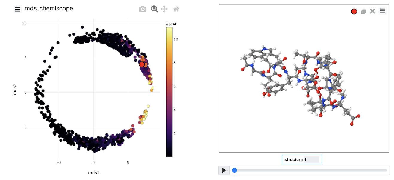
Try to generate an image that looks like this one yourself by completing the input above and then using what you learned about generating chemiscope representations in the previous exercise.
Sketch-map
The two algorithms (PCA and MDS) that we have looked at thus far are linear dimensionality reduction algorithms. In addition to these, there are a whole class of non-linear dimensionality reduction reduction algorithms which work by transforming the matrix of dissimilarities between configurations, calculating geodesic rather than Euclidean distances between configurations or by changing the form of the loss function that is optimized. In this final exercise, we will use an algorithm that uses the last of these three strategies to construct a non-linear projection. The algorithm is known as sketch-map and input for sketch-map is provided below:
# This reads in the template pdb file and thus allows us to use the @nonhydrogens # special group later in the inputMOLINFOThis command is used to provide information on the molecules that are present in your system. More detailsSTRUCTURE=__FILL__a file in pdb format containing a reference structureMOLTYPE=proteinwhat kind of molecule is contained in the pdb file - usually not needed since protein/RNA/DNA are compatible
# This stores the positions of all the nonhydrogen atoms for later analysis cc:COLLECT_FRAMES__FILL__=This allows you to convert a trajectory and a dissimilarity matrix into a dissimilarity object More details@nonhydrogens# This should output the atomic positions for the frames that were collected and analyzed using MDSall non hydrogen atoms. Click here for more information.DUMPPDB__FILL__=cc_dataOutput PDB file. More detailsATOM_INDICES=__FILL__the indices of the atoms in your PDB outputFILE=traj.pdbthe name of the file on which to output these quantities
# The following commands compute all the Ramachandran angles of the protein for you r2-phi:TORSIONCalculate a torsional angle. More detailsATOMS=the four atoms involved in the torsional angle@phi-2r2-psi:the four atoms that are required to calculate the phi dihedral for residue 2. Click here for more information.TORSIONCalculate a torsional angle. More detailsATOMS=the four atoms involved in the torsional angle@psi-2r3-phi:the four atoms that are required to calculate the psi dihedral for residue 2. Click here for more information.TORSIONCalculate a torsional angle. More detailsATOMS=the four atoms involved in the torsional angle@phi-3r3-psi:the four atoms that are required to calculate the phi dihedral for residue 3. Click here for more information.TORSIONCalculate a torsional angle. More detailsATOMS=the four atoms involved in the torsional angle@psi-3r4-phi:the four atoms that are required to calculate the psi dihedral for residue 3. Click here for more information.TORSION__FILL__ r4-psi:Calculate a torsional angle. More detailsTORSION__FILL__ r5-phi:Calculate a torsional angle. More detailsTORSION__FILL__ r5-psi:Calculate a torsional angle. More detailsTORSION__FILL__ r6-phi:Calculate a torsional angle. More detailsTORSION__FILL__ r6-psi:Calculate a torsional angle. More detailsTORSION__FILL__ r7-phi:Calculate a torsional angle. More detailsTORSION__FILL__ r7-psi:Calculate a torsional angle. More detailsTORSION__FILL__ r8-phi:Calculate a torsional angle. More detailsTORSION__FILL__ r8-psi:Calculate a torsional angle. More detailsTORSION__FILL__ r9-phi:Calculate a torsional angle. More detailsTORSION__FILL__ r9-psi:Calculate a torsional angle. More detailsTORSION__FILL__ r10-phi:Calculate a torsional angle. More detailsTORSION__FILL__ r10-psi:Calculate a torsional angle. More detailsTORSION__FILL__ r11-phi:Calculate a torsional angle. More detailsTORSION__FILL__ r11-psi:Calculate a torsional angle. More detailsTORSION__FILL__ r12-phi:Calculate a torsional angle. More detailsTORSION__FILL__ r12-psi:Calculate a torsional angle. More detailsTORSION__FILL__ r13-phi:Calculate a torsional angle. More detailsTORSION__FILL__ r13-psi:Calculate a torsional angle. More detailsTORSION__FILL__ r14-phi:Calculate a torsional angle. More detailsTORSION__FILL__ r14-psi:Calculate a torsional angle. More detailsTORSION__FILL__ r15-phi:Calculate a torsional angle. More detailsTORSION__FILL__ r15-psi:Calculate a torsional angle. More detailsTORSION__FILL__ r16-phi:Calculate a torsional angle. More detailsTORSION__FILL__ r16-psi:Calculate a torsional angle. More detailsTORSION__FILL__Calculate a torsional angle. More details
# This command stores all the Ramachandran angles that were computed angles:COLLECT_FRAMES__FILL__=r2-phi,r2-psi,r3-phi,r3-psi,r4-phi,r4-psi,r5-phi,r5-psi,r6-phi,r6-psi,r7-phi,r7-psi,r8-phi,r8-psi,r9-phi,r9-psi,r10-phi,r10-psi,r11-phi,r11-psi,r12-phi,r12-psi,r13-phi,r13-psi,r14-phi,r14-psi,r15-phi,r15-psi,r16-phi,r16-psi # Now select 500 landmark points to analyze fps:This allows you to convert a trajectory and a dissimilarity matrix into a dissimilarity object More detailsLANDMARK_SELECT_FPSSelect a of landmarks from a large set of configurations using farthest point sampling. More detailsARG=__FILL__the COLLECT_FRAMES action that you used to get the dataNLANDMARKS=500 # Run sketch-map on the landmarks smap:the numbe rof landmarks you would like to createSKETCHMAP__FILL__=fpsConstruct a sketch map projection of the input data More detailsNLOW_DIM=2number of low-dimensional coordinates requiredPROJECT_ALLif the input are landmark coordinates then project the out of sample configurationsHIGH_DIM_FUNCTION={SMAP R_0=6 A=8 B=2}the parameters of the switching function in the high dimensional spaceLOW_DIM_FUNCTION={SMAP R_0=6 A=2 B=2}the parameters of the switching function in the low dimensional spaceCGTOL=1E-3The tolerance for the conjugate gradient minimization that finds the projection of the landmarksNCYCLES=3The number of cycles of pointwise global optimisation that are requiredCGRID_SIZE=20,20number of points to use in each grid directionFGRID_SIZE=200,200interpolate the grid onto this number of points -- only works in 2D
# This command outputs all the projections of all the points in the low dimensional spaceDUMPVECTOR__FILL__=smap_osample.coord-1,smap_osample.coord-2Print a vector to a file More detailsARG=osamplethe input for this action is the scalar output from one or more other actionsFILE=smap_datathe file on which to write the vetors
# These next three commands calculate the secondary structure variables. These # variables measure how much of the structure resembles an alpha helix, an antiparallel beta-sheet # and a parallel beta-sheet. Configurations that have different secondary structures should be projected # in different parts of the low dimensional space. alpha:ALPHARMSDProbe the alpha helical content of a protein structure. More detailsRESIDUES=all abeta:this command is used to specify the set of residues that could conceivably form part of the secondary structureANTIBETARMSDProbe the antiparallel beta sheet content of your protein structure. More detailsRESIDUES=allthis command is used to specify the set of residues that could conceivably form part of the secondary structureSTRANDS_CUTOFF=1.0 pbeta:If in a segment of protein the two strands are further apart then the calculation of the actual RMSD is skipped as the structure is very far from being beta-sheet likePARABETARMSDProbe the parallel beta sheet content of your protein structure. More detailsRESIDUES=allthis command is used to specify the set of residues that could conceivably form part of the secondary structureSTRANDS_CUTOFF=1.0If in a segment of protein the two strands are further apart then the calculation of the actual RMSD is skipped as the structure is very far from being beta-sheet like
# These commands collect and output the secondary structure variables so that we can use this information to # determine how good our projection of the trajectory data is. cc2:COLLECT_FRAMESThis allows you to convert a trajectory and a dissimilarity matrix into a dissimilarity object More detailsARG=alpha,abeta,pbetathe arguments you would like to collectDUMPVECTORPrint a vector to a file More detailsARG=cc2_datathe input for this action is the scalar output from one or more other actionsFILE=secondary_structure_datathe file on which to write the vetors
This input collects all the torsional angles for the configurations in the trajectory. Then, at the end of the calculation, the matrix of distances between these points is computed, and a set of landmark points
is selected using a method known as farthest point sampling. A matrix that contains only those distances between the landmarks is then constructed and diagonalized by the CLASSICAL_MDS action, and this
set of projections is used as the initial configuration for the various minimization algorithms that are then used to optimize the sketch-map stress function. As in the previous exercise, once the projections of
the landmarks are found, the projections for the remainder of the points in the trajectory are found by using the PROJECT_POINTS action. This is managed by the SKETCHMAP shortcut action, however.
Try to fill in the blanks in the input above and run this calculation now using the command:
plumed driver --mf_pdb traj.pdb
Once the calculation has completed, you can, once again, visualize the data generated using chemiscope by using the scripts from earlier exercises. My projection is shown in the figure below. Points are, once again, coloured following the alpha-helical content of the corresponding structure.
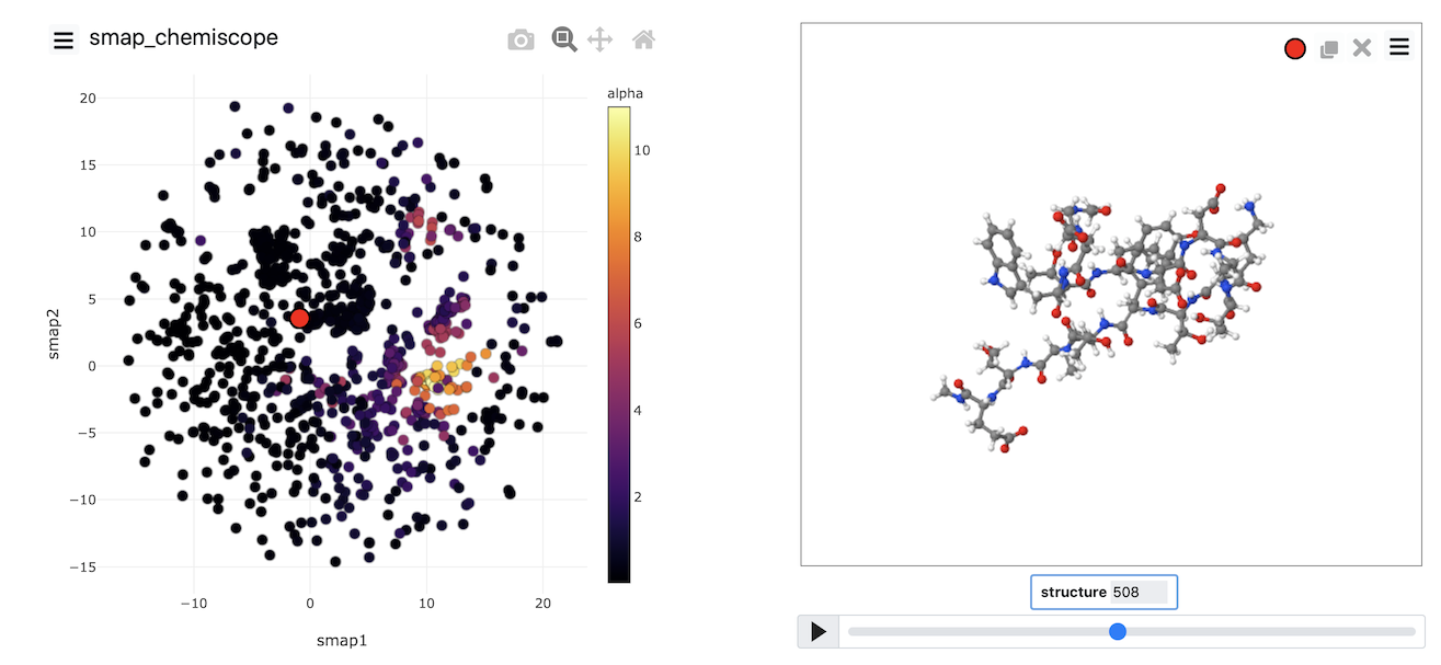
Try to see if you can reproduce an image that looks like the one above
Summary
This exercise has shown you that running dimensionality reduction algorithms using PLUMED involves the following stages:
- Data is collected from the trajectory using COLLECT_FRAMES.
- Landmark points are selected using a landmarks algorithm
- A loss function is optimized to generate projections of the landmarks.
- Projections of the non-landmark points are found
There are multiple choices to be made in each of the various stages described above. For example, you can change the particular sort of data this is collected from the trajectory. There are multiple different ways to select landmarks. You can use the distances directly, or you can transform them. You can use various loss functions and optimize the loss function using a variety of different algorithms. When you tackle your own research problems using these methods, you can experiment with the various choices that can be made.
Generating a low-dimensional representation using these algorithms is not enough to publish a paper. We want to get some physical understanding from our simulation. Gaining this understanding is the hard part.